NLP | Text Vectorization
How machines turn text into numbers to perform calculations
Machines can’t read text or look at images like us: they need their inputs to be transformed into numbers in order to perform calculations. Machine learning algorithms operate on a numeric feature space, even if they involve text data.
But how do you turn text into numbers?
Vectors and matrices represent inputs like text as numbers, so that we can train and deploy our models.
What is a vector?
When we use vectors as inputs, the main use is their ability to encode information in a format that our model can process, and then output something useful to our end goal. We can use vectors to represent the features we want our model to learn.
A vector is a list of numbers or a 1-D data structure
A vector is an object that has both a magnitude and a direction. Geometrically, we can picture a vector as a directed line segment, whose length is the magnitude of the vector and with an arrow indicating the direction. The direction of the vector is from its tail to its head.
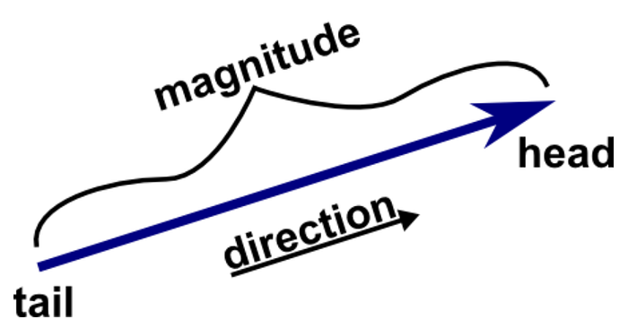

Vectors inhabit a space known as a vector space, in which we can manipulate them. Within this space, we can perform operations such as vector addition and multiplication.
When creating vectors based on text data, the results can be sparse (in which most features encode no information since they are empty, making them somehow “inefficient”), or dense (which contain very few or none zeros in any of the features).
As an example of dense vectors, the Universal Sentence Encoder (USE) model provides versatile sentence embedding models that convert sentences into vector representations.
Getting started
We must make a shift in how we think about language: from a sequence of words to points that occupy a high-dimensional semantic space. Points in space can be close together or far apart, tightly clustered or evenly distributed.
Semantic space is therefore mapped in such a way where documents with similar meanings are closer together and those that are different are farther apart. By encoding similarity as distance, we can begin to derive the primary components of documents and draw decision boundaries in our semantic space.
Bag of Words (BoW)
The simplest encoding of semantic space is the bag-of-words model, whose primary insight is that meaning and similarity are encoded in vocabulary. Here, documents are described by word occurrences while completely ignoring the relative position information of the words in the document.
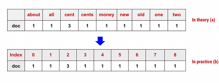
Scikit-learn’s CountVectorizer is used to convert a collection of text documents to a vector of term/token counts. Let’s see an example for the following phrases: “robots will augment humans”, “AI will affect human will”, and “humans will improve robots”:
from sklearn. feature_extraction. text import CountVectorizertexts = [“robots will augment humans”,
 “AI will affect human will”,
 “humans will improve robots”]vectorizer = CountVectorizer()
vectorizer.fit(texts)
print(vectorizer.vocabulary_)

Printing the identified unique words along with their indices provides the logic by which the model can be interpreted. The words have been arranged alphabetically, and converted to lowercase.
vector = vectorizer.transform(texts)
print(vector.shape)
The matrix has 3 rows (3 phrases), and 8 columns or unique words. Now let’s print our matrix:
print(vector.toarray())
Check row 2 (phrase “AI will affect human will”). The word “will” (indexed as 7, last position) appears twice.
Bow models have serious limitations. In the case of large documents, these models will extend over large dimensions resulting in sparse vectors. Also, BoW does a poor job in making sense of text data. For example, the sentences “I love robots and hate humans” and “I love humans and hate robots” will result in similar vectorized representations although both sentences carry totally different meanings.
Term frequency–inverse document frequency (TF-IDF)
The goal of TF-IDF is to avoid a common problem when conducting text analysis: the most frequently used words in a document are often the most frequently used words in all of the documents. In contrast, terms with the highest TF-IDF scores are the terms in a document that are distinctively frequent in a document, when that document is compared other documents.
TF-IDF models solve this problem by computing weights to each word which signifies the importance of the word in the document and corpus. They generate word frequency scores that try to highlight words that are more interesting, e.g. frequent in a document but not across documents.
Following the same steps as with BoW, we can calculate the TF-IDF matrix:
from sklearn.feature_extraction.text import TfidfVectorizer texts = [“robots will augment humans”,
 “AI will affect human will”,
 “humans will improve robots”]tfidf_vectorizer = TfidfVectorizer(use_idf=True)
tfidf_vectorizer.fit_transform(texts)
print(tfidf_vectorizer.vocabulary_)
tfidf_vector = tfidf_vectorizer.transform(texts)
print(tfidf_vector.toarray())

The score of the word “will” was significantly reduced due to its presence in all phrases, while the score of infrequent words like “augment” or “improve” went up. If a word appears very little or appears frequently, but only in one or two places, then these are probably more important words and should be weighted as such.
The scores are normalized to values between 0 and 1 and the encoded document vectors can then be used directly with machine learning algorithms like Artificial Neural Networks.
The problems with this approach (as well as with BoW), is that the context of the words are lost when representing them, and we still suffer from high dimensionality for extensive documents. The English language has an order of 25,000 words or terms, so we need to find a different solution.
Distributed Representations
With these models, the representation of a word is spread across all of the elements in the vector, and each element in the vector contributes to the definition of many words (each textual unit is encoded using a fixed length vector). Such a vector comes to represent in some abstract way the ‘meaning’ of a word.
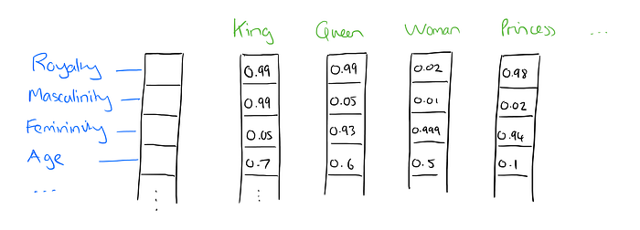
Word2vec implements a word embedding model that enables us to create these kinds of distributed representations. The basic idea is that words that occur in similar context tend to be closer to each other in vector space. The cosine similarity between the vectors indicates the level of semantic similarity between the words represented by those vectors.
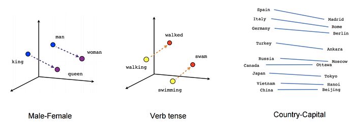
The model contains 300-dimensional vectors for 3 million words and phrases. It first constructs a vocabulary from the training text data and then learns vector representation of words.
Next, we will train our own Word2vec based on our 3 phrases:
from gensim.models import word2vectexts = [“robots will augment humans”,
 “AI will affect human will”,
 “humans will improve robots”]for i, text in enumerate(texts):
 tokenized= []
 for word in text.split(‘ ‘):
  word = word.split(‘.’)[0]
  word = word.lower()
  tokenized.append(word)
 texts[i] = tokenizedmodel = word2vec.Word2Vec(texts, size = 8, min_count = 1)
We defined the number of dimensions to be of 8, since that’s the total number unique words in our corpus. Based on this model, we can now perform tasks like word similarity:
model.most_similar(positive=['robots'], topn=1)The most similar word to “robots” is the word “ai”. Why? Because our model was trained based on our 3 phrases. That’s all it has seen so far.
How can we extend our vocabulary?
We are going to use Google’s pre-trained news model to expand our corpus. The model contains word vectors for a vocabulary of 3 million words trained on around 100 billion words from the google news dataset. The link to the dataset can be found here.
model2 = gensim.models.KeyedVectors.load_word2vec_format(‘GoogleNews-vectors-negative300.bin.gz’, binary=True)Now let’s see which are the 5 most similar word to “robots”:
model2.most_similar(positive=[‘robots’], topn=5)
You can see the model has a much larger lexicon, and also is case sensitive. What about the length of each vector?
len(model2[‘robots’])
Now we have 300 dimensions for each one of our vectors. Taking advantage of the extensive vocabulary, we can ask our model to give us the word that does not belong to a specific list:
print(model2.doesnt_match(“robots AI wine intelligence”.split()))
Word2vec has several advantages over BoW and IF-IDF models. It not only retains the semantic meaning of different words in a document, but also each dimension of the vector contains information about one aspect of the word (avoiding huge sparse vectors).
You can also visualize vectorized words in 3D with Word2vec in the TensorFlow Embedding Projector.

Conclusion
The task of language modelling has its own limitations: it’s only a proxy to true language understanding, and a single monolithic model is ill-equipped to capture the required information for certain downstream tasks. For instance, in order to answer questions about or follow the trajectory of characters in a story, a model needs to learn to perform anaphora or coreference resolution.
Language models can only capture what they have seen.
The secret to getting models really working for you is to have lots of text data in the relevant domain. For example, if your goal is to build a sentiment lexicon, then using a dataset from the medical domain or even wikipedia may not be effective.
So, choose your dataset wisely.
Since Word2vec, a lot of things have happened and the discipline is still evolving.
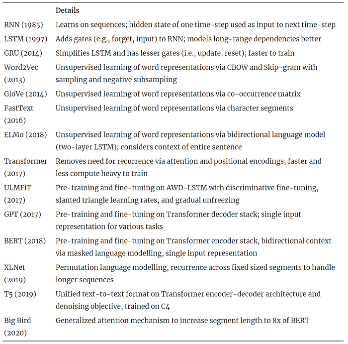
Today we are living in the age of Transformers, a Deep Learning arquitecture released in 2017 that revolutionized NLP by relying on self-attention mechanisms instead of recursion strategies. In the future, NLP will continue to transform how technology understands and assists us in ways that we can’t even imagine.
