Your guide to Perceptrons
The building blocks of Deep Learning

I’m sure you’ve heard about Deep Learning, and the awesome accomplishments this discipline has reached in the past years. Whether is solving protein structures or beating the South Korean Go champion Lee Se-dol (causing him to retire), Deep Learning has been all over the news recently.
What is Deep Learning?
Deep Learning is a subset of Machine Learning where Artificial Neural Networks (ANNs), which are algorithms inspired by the human brain, learn from large amounts of data.
Deep Learning uses a multi-layered structure of ANNs, enabling models to disentangle the kinds of complex and hierarchical patterns found in real-world data. This makes them so effective, that today they are used to solve tasks in a wide variety of fields such as computer vision (image), natural language processing (text), and automatic speech recognition (audio). Through their power, flexibility and scalability, ANNs have become the defining building blocks of Deep Learning. They represent components or pieces that “talk” to each other, and can be arranged in different ways to construct smart Deep Learning solutions.
What are Artificial Neural Networks (ANNs)?
ANNs are composed of neurons, where each neuron individually performs only a simple computation. The power of an ANN comes from the complexity of the connections these neurons can form. ANNs work in this way: they accept input variables as information, weight variables as knowledge, and output a prediction. Every ANN you’ll ever see works this way. They use the knowledge in the weights to interpret the information in the input data. This underlying premise will always remain true.
So, before getting into Deep Learning, it’s a good idea to begin with the fundamental component of an ANN: the individual neuron. A neuron returns some output information from several input data, and in the late 1950s, Frank Rosenblatt and other researchers developed a class of ANN called Perceptron.
The Perceptron algorithm is about learning the weights for the input signals in order to draw linear decision boundary that allows it to discriminate between two linearly separable classes. To make a decision whether a neuron fires or not.
The anatomy of a Perceptron
The Single-Layer Perceptron (SLP) has only one neuron, and sets the groundwork for the fundamentals of modern Deep Learning architectures. They perform classification tasks, and can deal only with linearly separable data.

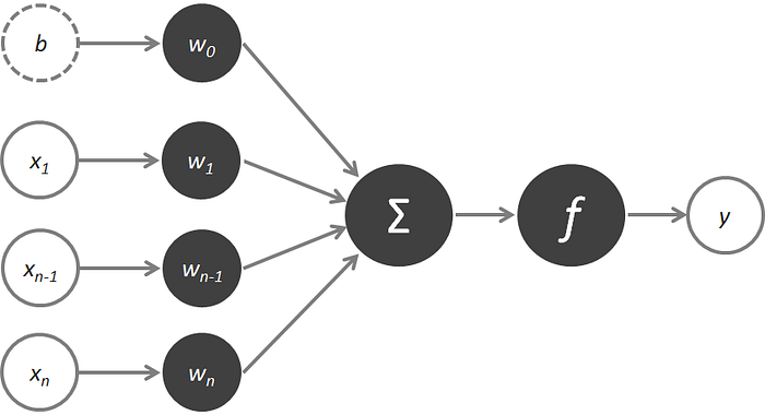
Look at the example above. The inputs of the SLP are x₁ to xn. Its connections to the neuron have weights which are w₁ to wn. Whenever a value flows through a connection, you multiply the value by the connection’s weight. For the input x₁, what reaches the neuron is x₁ * w₁ . An ANN "learns" by modifying these weights: a low weight will de-emphasise a signal, and a high weight will amplify it.
The b is a special kind of weight called the bias. The bias doesn’t have any input data associated with it, and enables the neuron to modify the output independently of its inputs.
The Σ represents the input function, or weighted average sum in this case.
The f represents the activation function which is the decision making unit of an ANN.
An activation function is a function that takes an input signal and generates an output signal, taking into account some kind of threshold.
The heaviside step function (also called unit step function) is the most common activation functions in these type of ANNs, which produces binary outputs. This function produces 1 (true) when the input passes certain threshold limit θ, or a 0 (false) otherwise, which makes it very useful for binary classification problems.

Finally, the y is the value the neuron ultimately outputs. To get the output, the neuron sums up all the values it receives through its connections.

In summary, a SLP receives multiple input signals, and if the sum of the input signals exceed a certain threshold, it either returns a signal or remains “silent” otherwise. It multiplies inputs by weights, sums those results, then “scales” that sum by a certain amount and produces an output.
How do Perceptrons learn?
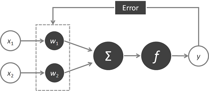
Once the SLP makes a prediction, the next step is to evaluate how well it did. Given a prediction, we want an error measure that states either that we missed by “a lot” or by “a little”. And after our errors are captured, the next step is to learn using some learning rule.
A learning rule is a procedure for modifying the weights and biases of the ANN. The purpose of the learning rule is to train the ANN to perform some task, optimizing its performance. Although there are many ways to measure error, the SLP uses the Mean Squared Error (MSE) as the function to estimate how well it did on each iteration.
Using a learning rule, the ANN outputs are compared to the targets, and the learning rule is then used to adjust the weights and biases of the ANN in order to move the outputs closer to the targets. How? The process works like this:
- The weights are initialized with random values at the beginning of the training.
- For each element of the training set, the error is calculated with the difference between the desired and the actual output. The error calculated is used to adjust the weights.
- The process is repeated until the error level over the training set reaches a specified threshold, or until a maximum number of iterations is achieved. Through this iteration, the Perceptron changes the weight (up or down) to predict more accurately the next time it sees the same input.

The learning process is about error attribution, the art of figuring out how each weight played its part in creating error. Learning in ANNs is a search problem: you’re searching for the best possible configuration of weights so the network’s error falls as closer to 0 as possible.
The weight vector is a parameter to the SLP: we need to tweak it until we can correctly classify each of the inputs.
Can we determine an appropriate way of modifying the weights optimizing the iteration?
First, we need to define the error (e) , and we can do it as the difference between the desired output yₜ (target) and the predicted output y.

Notice that when yₜ and y are the same, the error equals 0, but when they are different, we can get either a positive or negative value. This directly corresponds to exciting and inhibiting the SLP, which means we can multiply this result with the input to tell the SLP to change the weight vector in proportion to the inputs.
Finally, we need to define a learning rate (l), which is a scaling factor that determines how large or smooth the weight vector updates should be. It moderates the updates to the weights, calming them down a bit. Why?Training examples from the real world can be noisy or contain errors, so moderating updates limits the impact of these false examples.
The learning rate (l) is called a hyperparameter because it is not learned by the SLP, since there’s no update rule for it.

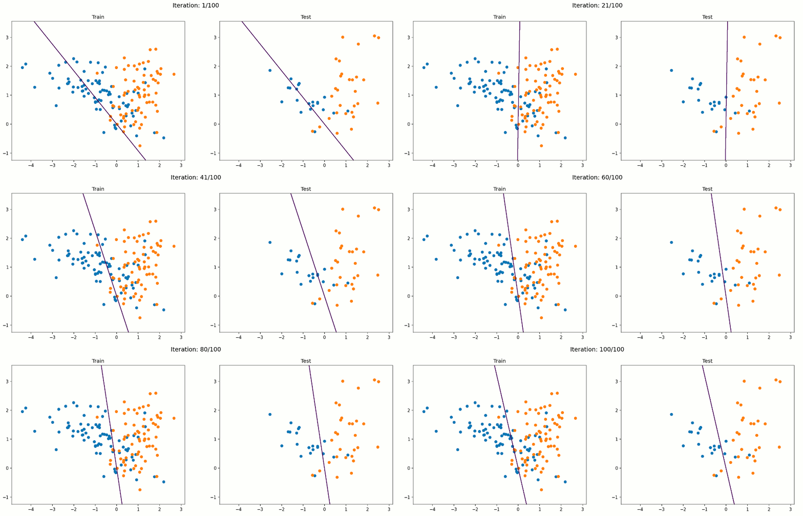
In geometrical terms, the learning goal of a SLP like the one detailed before is to adjust the separating hyperplane that divides an n-dimensional space, where n is the number of input units (+ 1), by modifying the weights and bias until all of the examples with target value 1 are on one side of the hyperplane, and all of the examples with target value 0 are on the other side of the hyperplane.

Limitations of the SLP
SLPs represent weak models because they can only learn linearly-separable functions, and as we know, the world is generally non-linear. They also output diverse results on different runs, since all they care about is reaching some linear discrimination, not necesarily the most optimal one. Because of this, they are deeply affected by the order in which they process the data registers. SLPs stop learning when they stop making mistakes, and there can be multiple weight vector and combinations at which no mistakes occur.
The good news is that you can use multiple linear classifiers to divide up data that can’t be separated by a single straight dividing line.
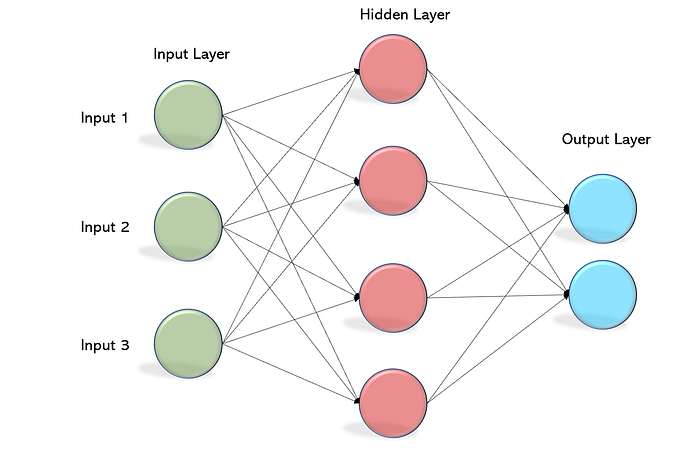
It was not until the 1980s that some of the these limitations were overcome with an improved concept called Multi-Layer Perceptron (MLP). MLPs were found as a solution to represent nonlinearly separable functions, where the outputs of one layer are the inputs of the next one.
MLPs consist of three types of layers: the input layer, the output layer and one or more hidden layers. The input layer receives the input signal to be processed on one side, and the required task (e.g. classification) is performed by the output layer on the other side. The hidden layers placed in between the input and output layer are the true computational engine of the MLP.

Today the SLP is still considered an important ANN, since it remains a fast and reliable algorithm for the class of problems that it can solve, and provides a good basis for understanding more complex ANN architechtures.
